Descartes' Rule and Viro Diagrams.

Descartes' Rule

We start with univariate polynomials. We assume numerical polynomials which implies, among other things, that no coefficient is exactly zero and there are no exact multiple zeros. Descartes' rule can be formulated in the following combinatorial and visual way:

Assign to a polynomial f = a₀+a₁x+ ...+a_dx^d a list {s₁, s₂, ..., s_d+1} where s_j is zero if a_j-1 is positive, and 1 if a_j-1 is negative, zero not being allowed. Note: the index shift and some other notation is because I use Mathematica and it is more important to make coding easier than to make reading this document easier. Note

f = (-1)^s₁|a₀| + (-1)^s₂|a₁|x +(-1)^s₃|a₂|x²+ ... +(-1)^s_d+1|a_d|x^d
We draw a diagram as follows: On a horizonal axis put a green dot at j-1 if s_j is 0, i.e. a_j is positive and a red dot otherwise. For positive j if j is even at -j use same color dot, if j is odd use opposite color. Finally draw a piecewise curve over the green dots and below the red dots as shown:

The first picture is of a polynomial such as

f= 1.34-2.56 x + 3.14x² +5.43 x³-0.8x⁴ while the second is a degree 8 polynomial with s={0,1,0,1,0,0,1,1,0}.

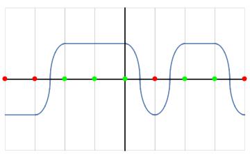
Descartes' rule then counts the possible number of postive and negative zeros, that is the number of times the graph would cross the x-axis on the positive side and on the negative side. Notice the total is always the degree.

Descartes' RuleThe number of positive zeros differs from the number of times the curve in the diagram crosses the axes on the positive side by an even number but is never more than shown in the picture. Likewise the number of even zeros is bounded by the curve in the diagram and differs by an even number.

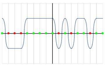
So in the first diagram there can be 3 or 1 positive zeros and must be exactly 1 negative zero for this 4th degree polynomial. In the second diagram there may be 6,4,2 or 0 positive zeros and 2 or 0 negative zeros for this 8th degree polynomial.

Viro Diagrams

The 2-dimensional version of this will be called a Viro Diagram after Oleg Viro, a contemporary, to this author, Russian mathematician, who proposed this idea in 1979.

Now we have a bivariate polynomial which is a finite sum

f(x,y) = a_0,0 + a_1,0x + a_0,1y + a_2,0x² + a_1,1x y + a_0,2y²+ ...

where for each monomial a_j,kx^jy^k the exponent is the pair {j,k} and the degree is j+k. The total degree of this polynomial is the highest degree of a monomial. The solution f(x,y) = 0 for x,y real, is no longer a set of points but a real algebraic plane curve. The goal is to now count the number of points where the curve crosses from one quadrant of the real projective plane to another where the quadrants are given, as in beginning algebra, by

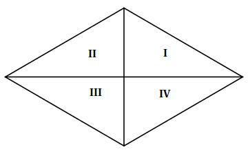
except that diagonal lines here refer to the projective infinite line and a curve can cross the infinite line from quadrant I to quadrant III and quadrant II to quadrant IV, that is, a curve can cross from any quadrant to any other. We want to count each kind of crossing.

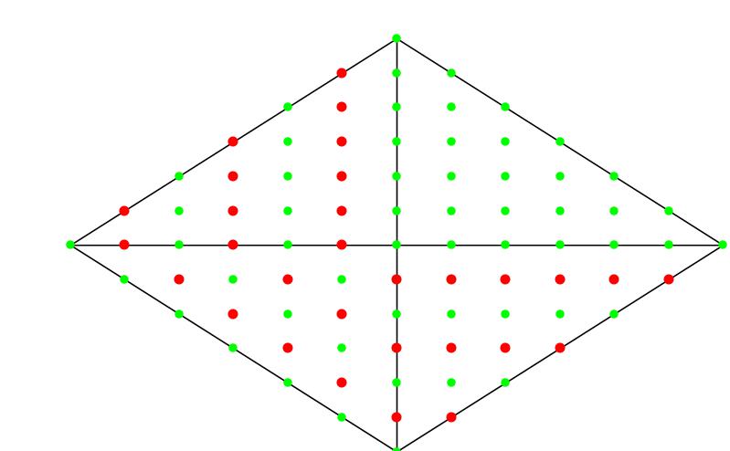
We proceed as in Descartes' rule except here we label the exponent {j,k} in quadrant I with with a green dot if the coefficient of x^jy^k is positive and with a red dot if the coefficient is negative. The idea of plotting the exponents on a plane lattice goes back to Newton but he used the condition 0 or not 0 on the coefficient generating the Newton Polygon which is still an important concept in computational algebra. This is extended to a plane rhombus by, as in Descartes's rule labeling {-j,k}, j,k > 0 the same as {j,k} if k is even and the opposite color. A similar rule is used for {j,-k}. For {-j,-k} use same color if j,k, have the same parity and opposite color if j,k, have opposite parity. This pattern becomes clear if we start with all positive coefficients:

Again we describe the configuration of dots by a binary sequence where a green dot gets 0 and red dot gets 1 with exponents in the following degree-lex order: {{0,0},{1,0},{0,1},{2,0},{1,1},{0,2},{3,0},{2,1},{1,2},{0,3}...} The length of the binary sequence must be 3,6,10,15,21,28,36,45 for my software to work, that is, curves up to degree 8.

Finally we consider two dots of the same color in the same component if the exponents agree in one direction and differ by 1 in the other. Following Gauss (Chapter 4 of curve book) we draw continuous curves bounding the components where the curves intersect horizontal and vertical integer lines at points {m,.5} or {.5,n} for m,n integers. For example when s= {0,1,0,0,1,0,1,1,0,0} the Viro Diagram looks like

Notice the one square between {0,0} and {1,-1}

is indeterminant, that is it would make sense if either the dotted cyan segments were used or the dotted magenta segments. In the first case the green components in the third and 4th quadrants would be one green connected component, in the second we would have one red component spanning the first and fourth quadrants.

The sign sequence alone will not determine which of the above is correct, in fact, a small perturbation, not affecting coefficient signs, of an actual curve with the topology on the left will give a curve with the topology on the right. So our software gives the indeterminant choice by default but the user can specify either specific choice. Topologically the left represents a projective curve with one pseudo-line A → C → B → A while the right represents a curve with two components: a pseudo-line A → A and an oval B → C → B.

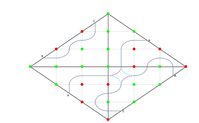
The analogue of Descartes' Theorem for Viro Diagrams is that for a curve with the given sign sequence the number of passages from one quadrant to another is bounded by the number of passages in the corresponding Viro Diagram and differs from the diagram along each boundary by an even number (sometimes stated "agrees modulo 2").

Note that the presence of indeterminant squares does not affect the number of quadrant changes. So regardless of the choice there must be one passage from the first quadrant to the third, one or 3 from first to fourth and also third to fourth and 2 or no passages from second to fourth. In partcular a curve with this sign sequence could have the right hand choice with no oval. But, of course, the pseudo-line is required of any cubic.

It should be noted that from the two dimensional Descartes' Rule point of view only the dots on the boundary count. In fact, for the horizontal and vertical axes the analogue of the one dimensional case follows directly from that case by setting one of the variables to 0. The case of passage across the infinite line but relys on the calculation of infinite points from the maximal form f_max and replacing x by a large positive constant. The internal dots may still be useful in seeing how it is possible for the curve to look between the quadrant boundaries. Ovals of the Viro Diagram lying entirely in some quadrant may or may not exist for a specific curve with these sign changes. Actually, Viro's interest in these diagrams was the converse starting with the diagram. He was interested in knowing if a curve with the topology of the diagram could actually exist with given sign sequence. He proved that in fact such a curve does exist but did not give explicit coefficients. We cannot do that either in general, but we can in specific cases.

Newton Hyperbolas

Newton was interested in cataloging real cubic functions [See D.J. Struik, A Source book in Mathematics 1200-1800, Princeton, 1986, pp. 162--178], he called them hypberbolas because of the asymptotes. I have generated a numbered list of approximately 2²⁸ curves up to degree 6 with many asymptotes which I call, in honor of Newton's work sometime between 1676 and 1704 on real cubics. These curves have the property that they maximize the number of quadrant changes in the Viro Diagrams of their sign sequence. In general they may not have all the ovals in the diagrams which are contained in a quadrant. Software for calculating Newton Hyperbolas, at least up to degree 4, is available on this website.

But these Newton Hyperbolas can be used as a starting point to finding a curve which does have the same topology as a Viro Diagram. We give several examples.

We start with the Viro diagram for s= {0,1,0,0,1,0,1,1,0,0} pictured above which corresponds to the sign sequence for Newton Hyperbola 210 (NH210).

f = 1 - x + y + 0.2x² - xy + 0.2y² - 0.008x³ - 0.2x²y + 0.2xy² + 0.008y³ A Mathematica region plot shows the positive region of this function (shaded light blue) with boundary being the curve with the modified Viro Diagram choosing the cyan path next to it (red region is negative corresponding to white region of the region plot).

While at this scale it is a little hard to see that this curve crosses the x-axis at approximately 1.33975,5.0 and 18.6603 ending slightly below the x-axis but Descartes Rule is satisfied at the maximum. The asymptote is actually in quadrants IV and II. Likewise this curve crosses the y-axis at -1.33975, -5.0 and -18.6603 leaving the asymptote also in quadrants II and IV. It appears, and this is correct, that there is one asymptote in quadrants I and III. Thus we see that topologically the curve NH210 matches the Viro Diagram.

However we can make the positive region smaller by making the constant term smaller, 0.3, but keeping it positive thus preserving the sign sequence. As noted above this does not change the passages across quadrants.

We now see the topology matches the Viro Diagram with the magenta choice. Thus we can match either of the variants of the Viro Diagram with an algebraic curve, up to topology. But since the change in function is fairly small with no change in sign sequence we also see why diagrams like this must come with indefinite squares.

We now shift gears from one of the easiest examples to the hardest. When Harnack stated his curve theorem in 1876 he claimed to have maximal examples (called M curves) for each degree, i.e. a curve of degree d with (d-1)(d-2)/2+1 connected projective components. Viro gives a recipe for the diagram. Here is a slightly modified Newton Hyperbola friendly version constructed inductively by d: Begin with a green dot at {0,0}. For the next diagonal starting at {n,0} if n is odd fill the diagonal with red dots, if n is even start with a green dot and then alternate red and green ending in green. For example for d= 3,4,5,6 we have

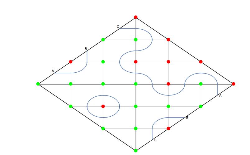
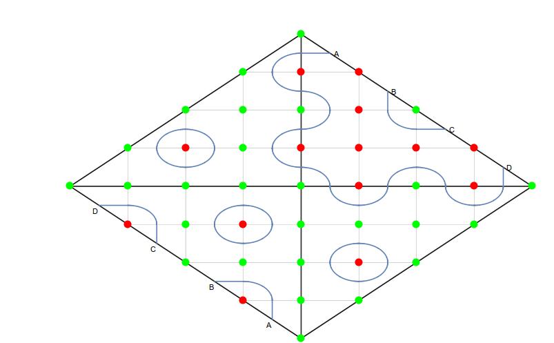
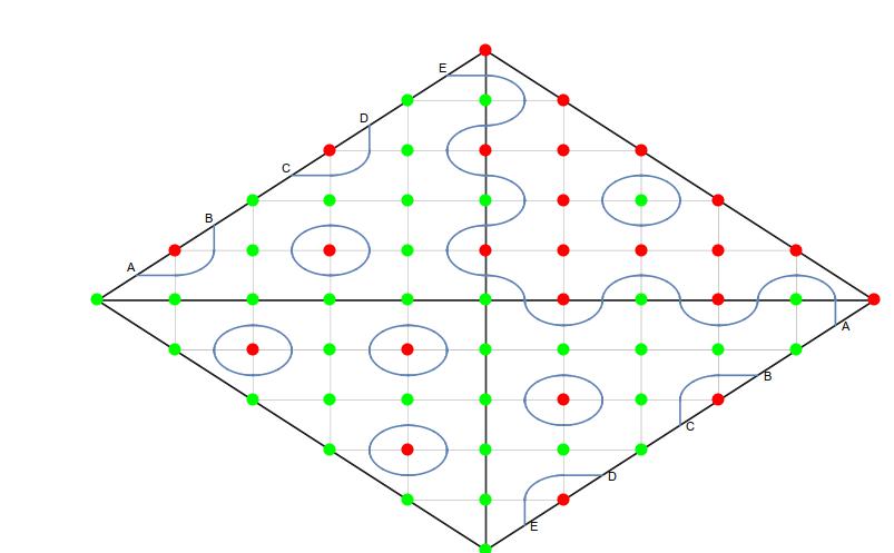
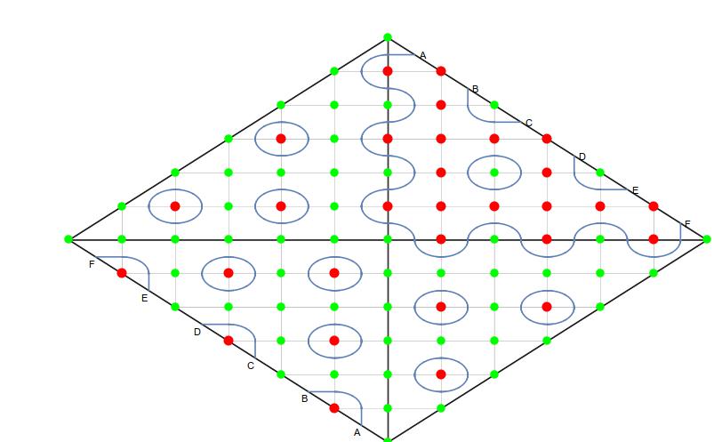
In each case there is one big component which intersects the infinite line in d places and (d-1)(d-2)/2 finite ovals.

Unfortunately, the Newton Hyperbolas which have the correct sign sequences give only the big component. These are NH982, NH11222, NH2075606, NH90155990 respectively. In the case of d=3 and d=4 it is relatively easy to modify the Newton Hyperbola to get a curve fulling matching the Viro Diagram.

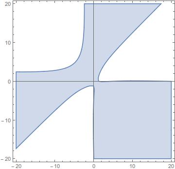
For d=3 we take NH982 - 4xy = 1 - x - y + 0.2x² - 5xy + 0.2y² - 0.008x³ - 0.2x²y - 0.2xy² - 0.008y³.

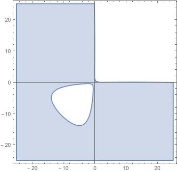
Comparing the Viro Diagram with a Mathematica Region Plot, again the red area of the Viro Diagram corresponds to the white area in the region plot. Also the pieces of the big component in quadrants II and IV are not shown as they are far from the plot region.

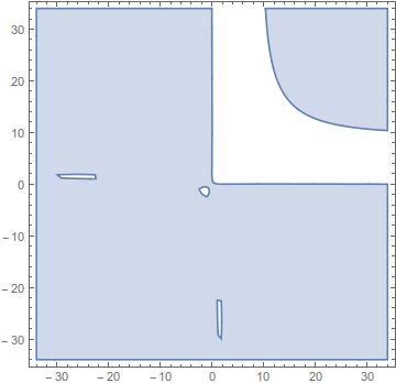
For d=4 we take NH11222 - 6xy - xy² - x²y. Here our region plot shows the 3 finite ovals and pieces of the big curve in the first quadrant but again the third quadrant pieces of the big curve are out of the plot range. Here the 4 white areas are interiors of the ovals.

Of course these curves are not exciting as there are simpler known examples of M-curves in degree 3 and 4. I will leave it to my readers to work out explicit actuations of curves matching the Viro Diagrams for d=5,6 starting from NH2075606 and NH90155990 respecively and preserving their sign sequences. These would be exciting and I will give the first people to get a correct equation credit on my website and/or book.